

How To Change Axis Range In Excel
How to customize chart axis
Author: Oscar Cronquist Article last updated on February 17, 2021
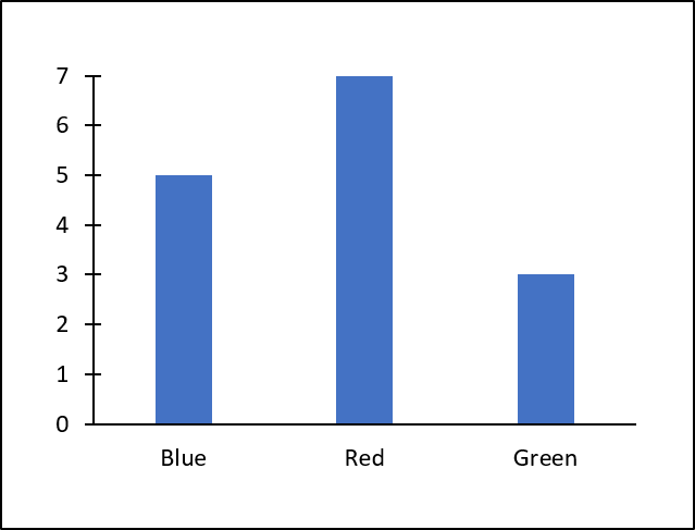
Most Excel charts consist of an x-axis and a y-axis, Excel allows you to easily change the looks of the chart axis.
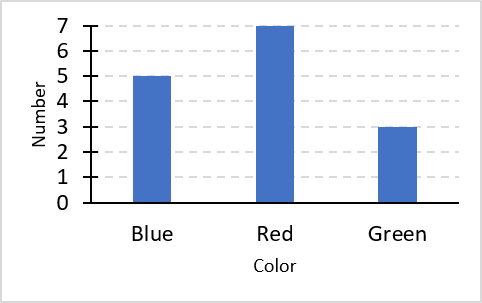
The chart below is what Excel returns using a few random values as a data source, there are, however, no axis lines.
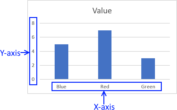
I have drawn a blue rectangle surrounding each group of axis values in the chart above.
To make it easier to see the changes I am about to do, I am now going to remove the major horizontal grid lines.
Simply press with left mouse button on the gridlines and press delete on your keyboard to remove them.
Font size of axis values
Axis value font type
Axis value font color
Customize axis line
Axis line tick marks
Tick marks interval
Axis line position
Add axis title text
Font size of axis values
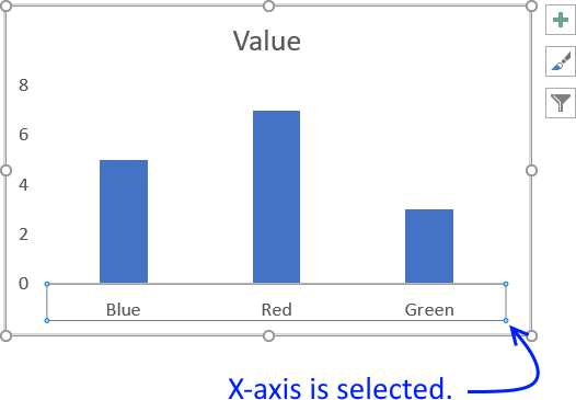
To change the font size of the axis values select the axis you want to change.
Go to tab "Home" on the ribbon then press with left mouse button on font size.
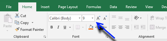
I chose font size 16.
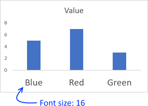
Tip! If you want to quickly format the y-axis with the same font size, follow these steps.
- Select the x-axis.
- Go to tab "Home" on the ribbon.
- Press with mouse on "Format Painter" button.
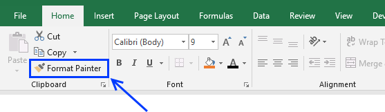
- Press with mouse on y-axis.
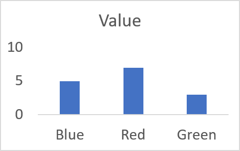
Both chart axis now have the same font size, this technique can be used on many different Excel objects, not only charts.
Back to top
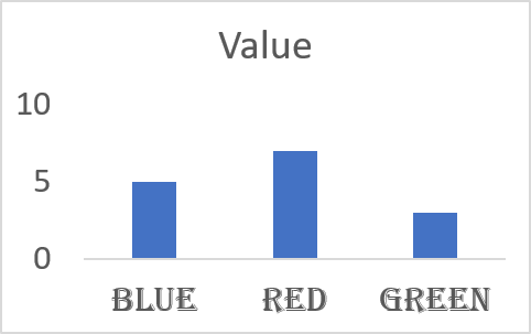
Axis value font type
- Press with mouse on the axis values you want to change.
- Go to tab "Home" on the ribbon.
- Press with mouse on font.
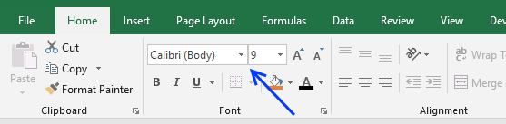
- Select a font.
Back to top
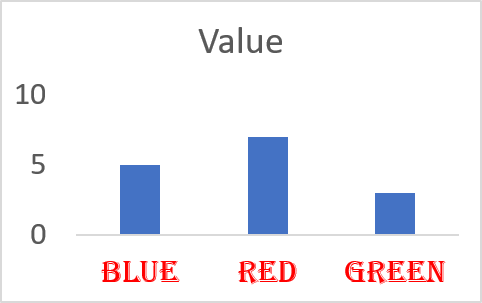
Axis value font color
- Select axis values
- Press with mouse on font color button.
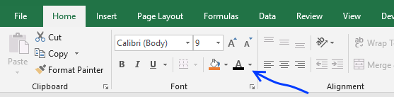
- Pick a font color.
Back to top
Customize axis line
- Press with right mouse button on on x-axis values.
- Press with mouse on "Format Axis..."
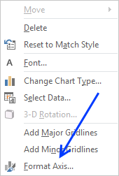
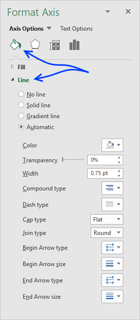
- Press with mouse on the "Fill and Line" button.

- Press with mouse on Line to expand the Line settings
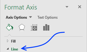
- Now you can change the color of the axis line, thickness, dashed or dotted and so on.
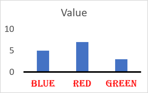
I exaggerated the axis line thickness and changed the color black to make it stand out.
Back to top
Axis line position
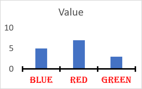
- To change the position of the x-axis you must press with right mouse button on on the y-axis and vice versa.
- Press with mouse on "Format Axis..."
- Press with mouse on the "Axis Options" button.
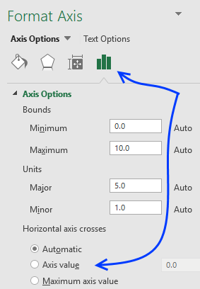
- Find Horizontal Axis crosses and select Axis value.
- Change it to the value on the y-axis you want the x-axis to cross, or vice versa.
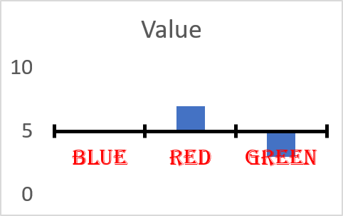
Back to top
Add axis title text
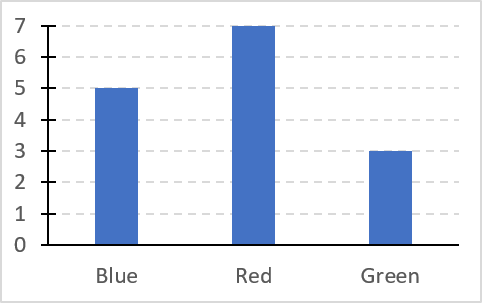
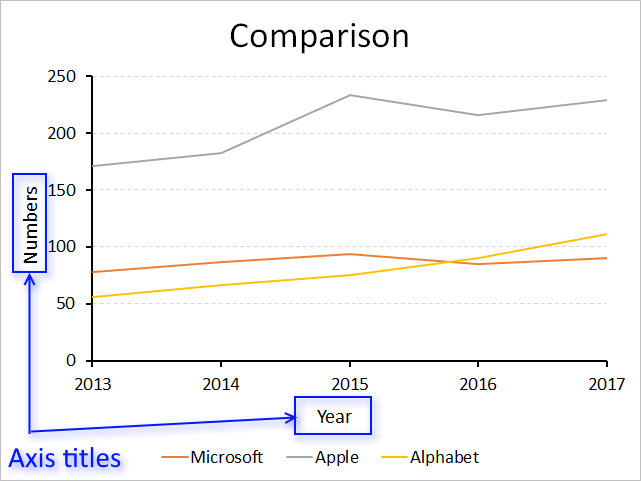
The chart above has no descriptive titles, follow these simple steps to add chart axis titles.
- Select chart.
- Go to tab "Design" on the ribbon. The tab will appear as soon as you select the chart.
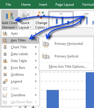
- Press with mouse on "Add Chart Element".
- Press with left mouse button on "Axis Titles".
- Press with mouse on "Primary Horizontal" or "Primary Vertical"
Back to top
Two y-axes in one chart
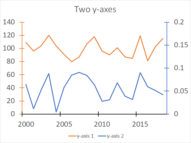
The image above demonstrates a line chart containing two data series and two y-axes, one for each data series. I […]
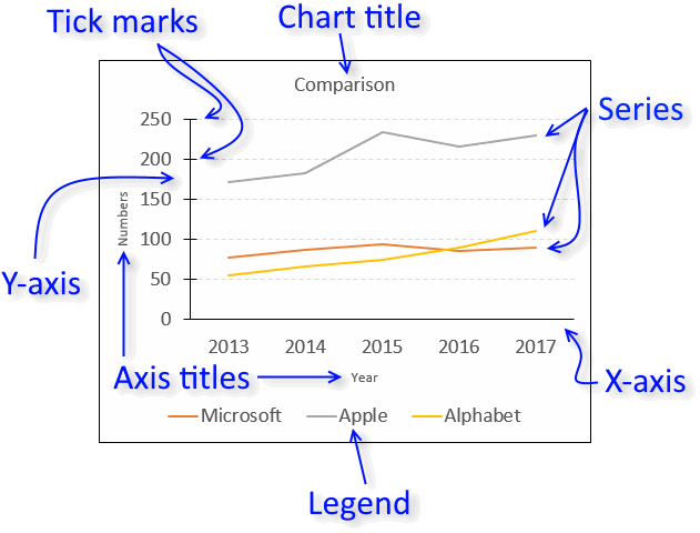
Excel chart components
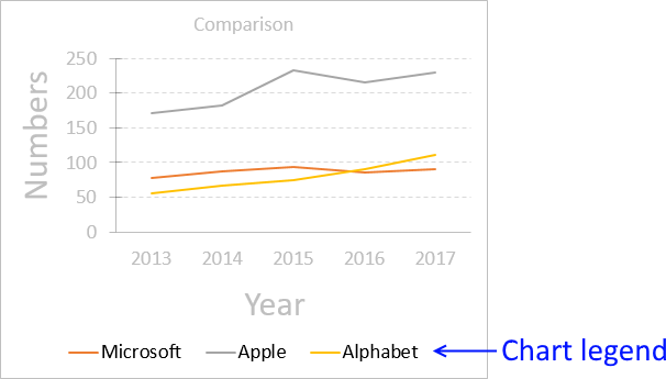
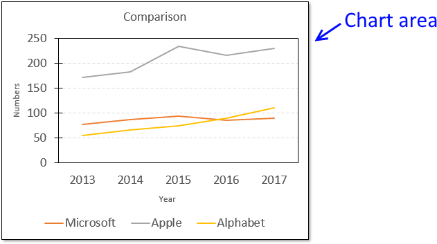
Charts in Microsoft Excel lets you visualize, analyze and explain data. Charting in Excel is very easy and you […]
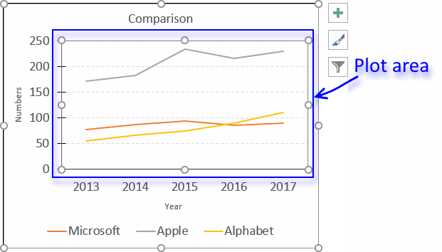
How to customize the plot area
The plot area refers to the location of the chart that displays the actual data represented by lines, bars, columns, […]
How To Change Axis Range In Excel
Source: https://www.get-digital-help.com/how-to-customize-chart-axis/
Posted by: watkinsparented58.blogspot.com
0 Response to "How To Change Axis Range In Excel"
Post a Comment